Canavan Disease: Task 10 - Normal Mode Analysis

Normal Mode Analysis is a way to predict the dynamics behind a protein. Here elastic network models are used, since they are very memory reducing.

Background

There are several servers available, which can give some indication of the movement and dynamics within the protein. There are three main approaches to do this:

• Molecular Dynamics (MD)
• Normal Mode Analysis (NMA)
• Elastic Network Models

In Molecular Dynamics ...
Using Normal Mode Analysis the slow motions of a protein can be investigated. It is important to know that normal modes with the lowest frequencies (soft modes) are those representing the movements.
Elastic Network Models ...
To sum it up, What are the advantages and disadvantages of NMA compared to MD?

For this Task two servers WEBnm@ and NOMAD were used to calculate normal modes of aspartoacylase using the pdb-structure 2O4H. The severs provide different possibilities calculating the nomal modes. The next <xr id="servers"></xr> should give an overview of the differences and similarities between the servers:

<figtable id="servers">

Differences and Similarities in WEBnm@ and NOMAD
Comparison	Webnm@	NOMAD
Background (see References)	WEBnm@ is using the MMTK package: MMTK calculates the low-frequence domain movements using an approximate normal mode calculation method by Hinsen et al. 200 modes are calculated for proteins with less than 1200 residues. Proteins with more than 1200 residues (N>1200) will bring N/6 modes. Only the lowest frequency modes should be taken into account. Therefore WEBnm@ presents the modes 7-12 to its users.	NOMAD makes its calculation using Elastic Network Models (or classical force fields): The Elastic Network Models (ENM) bring the advantage that a prior energy minimization to find the eigenvectors in the Hessian Matrix is not needed. The ENMs represent a set of harmonic potentials between atoms. This state represents the global minimum. Up to 160 modes are allowed to be calculated. The user has the possibility to choose how many modes.
	Calculation implies the use of the Hessian Matrix, since its eigenvectors represent the normal modes. The first 6 (zero-frequency) modes represent the global rotation and translation of the protein
Which part of the structure is taken into account for the calculation?	C-alpha atoms only
	-	2 further options: all atoms, sidechains only
Which analysis tools are available?	visualization, fluctuations, eigenvalues
	deformation energies, atomic displacements, correlation matrix	frequencies, overlap coefficients, structure minimization using GROMACS (only structures with less than 3000 atoms)
What options do I have?	choosing chain of protein, Comparative Analysis	Number of modes to calculate (first six ones are translation and rotation), distance weight (for elastic constant), ENM Cutoff (for mode calculation), Average Rmsd (in output trajectories)

Comparison of the servers WEBnm@ and NOMAD.

</figtable>

WEBnm@

• Which regions of your protein are most flexible, most stable?
• Try the comparison/upload of second structure option, if: (i) you have PDB structures in different conformations or (ii) your protein has a bound ligand. Then either upload a structure with and one without the ligand, or delete the ligand in your structure.
• For WEBnm@ try the amplitude scaling and vectors option.

</figure>

</figure>

</figure>

text.

text.

text.

<figure id="eigenvalues">

<figure id="correlation">

<figure id="correlation">

</figure>

</figure>

</figure>

</figure>

</figure>

</figure>

</figure>

</figure>

</figure>

</figure>

</figure>

</figure>

text.

text.

text.

text.

text.

text.

text.

text.

text.

text.

text.

text.

Mode 7: Deformation Energy: 890.47 text (hinge-movement, “breathing”… )	<figure id="mode7">
<figure id="mode7plot">
Mode 8: Deformation Energy: 1001.20 text	<figure id="mode8">
<figure id="mode8plot">
Mode 9: Deformation Energy: 1576.14 text	<figure id="mode9">
<figure id="mode9plot">
Mode 10: Deformation Energy: 2832.63 text	<figure id="mode10">
<figure id="mode10plot">
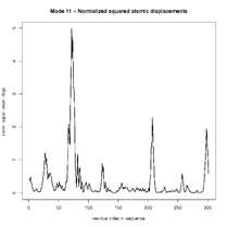
Mode 11: Deformation Energy: 2837.90 text	<figure id="mode11">
<figure id="mode11plot">
Mode 12: Deformation Energy: 2995.56 text	<figure id="mode12">
<figure id="mode12plot">

NOMAD

Since there was a problem using the server, elNemo could not be taken into account. Therefore NOMAD was chosen to predict normal modes.

• Visualize some modes (provided by server or using for example PyMol or VMD). Choose between 2-10 modes you believe are interesting and describe what movements you observe: hinge-movement, “breathing”…
• Which regions of your protein are most flexible, most stable?

</figure>

</figure>

</figure>

</figure>

</figure>

</figure>

</figure>

</figure>

</figure>

</figure>

</figure>

</figure>

text.

text.

text.

text.

text.

text.

text.

text.

text.

text.

text.

text.

Mode 7: The motion of the protein completely centres around the binding pocket. Overall it is a seesawing motion of all parts towards the centre with the most flexible part being the lower left loop region. The secondary structure elements are the most rigid parts.	<figure id="mode7">
<figure id="mode7plot">
Mode 8: In mode 8 a hingelike motion is detectable, that is centring around the active site of the protein, and looks like a clamming of the protein to the potential substrate. The outer loopregions are the most flexible parts of the protein, whereas the secondary structure elements are the most stable.	<figure id="mode8">
<figure id="mode8plot">
Mode 9: Mode 9 is sort of a combination of the clamming movement of mode 8 and the seesaw movement of mode 7. Again the motion seems centred around the binding pocket of the protein.	<figure id="mode9">
<figure id="mode9plot">
Mode 10: This mode has like mode 8 a hinge like motion with the difference to mode 8 being that he imaginary plane that defines the hinge movement is orientated differently. As with the other modes the motion is centred around the binding pocket and the most flexible part is the loop region in the bottom left.	<figure id="mode10">
<figure id="mode10plot">
Mode 11: The motion of model 11 is best described as if two planes of the protein are moved into opposite directions. Centre of the motion, the most flexible and rigid parts of the protein are the same as with the other modes.	<figure id="mode11">
<figure id="mode11plot">
Mode 12: Mode 12 combines the clamming motion of mode 8 and 10 with a breathing of the protein. Interpreting this motion tends to give the same result as before, with motion surrounding the active site, and the loop regions being the most flexible.	<figure id="mode12">
<figure id="mode12plot">

Comparison

• Can you observe notable differences between the normal modes calculated by the different servers?
• Compare with SCOP and Pfam

References

official papers:

• WEBnm@
• NOMAD

Tasks

• Link to Task 01: Canavan Disease
• Link to Task 02: Alignments
• Link to Task 03: Sequence-based Predictions
• Link to Task 04: Structural Alignments
• Link to Task 05: Homology Modelling
• Link to Task 06: Protein Structure Prediction from Evolutionary Sequence Variation
• Link to Task 07: Researching SNPs
• Link to Task 08: Sequence-based Mutation Analysis
• Link to Task 09: Structure-based Mutation Analysis
• Link to Task 10: Normal Mode Analysis