Hemochromatosis Normal modes
Labjournal_NMA-Hemochromatosis
Contents
Introduction
<figure id="timescale">
</figure>
TODO for what do we use NMA? -> reference to <xr id="timescale"/>
WebNMA and elNemo are two different web servers for normal mode analysis. Both provide different information:
- WebNMA
- normal modes + animations
- average residue fluctuations
- correlated residue movement map
- elNemo
- normal modes + animations
- average residue fluctuations
- pairwise correlated residue movement as a list
The modes are only calculated from the C-alpha atoms of the proteins residues. In principal, 3N-6 normal modes could be computed, where N is the number of atoms in the molecule. The reasoning behind this number is, that each atom in a molecule has three coordinates and the molecule thus has 3N degrees of freedom. However, three degrees of freedom have to be omitted to account for translation and another three have to be omitted to account for rotational symmetry. For the HFE protein with 272 residues, 810 normal modes can be calculated, but only the low frequency normal modes are of interest, because they resemble slow motions.
elNemo
<figure id="elnemo">
</figure>
<xr id="elnemo"/> shows the five most most interesting and distinct normal modes of the HFE protein. The first six are omitted because they are of low complexity.
WebNM@
<css> table.basic2 { margin-left: auto; margin-right: auto; border: 0px solid black; border-collapse:collapse; width: 20%; }
.basic2 th,td { padding: 3px; border: 1px solid black; }
.basic2 th { border-bottom: 2px solid black; background-color: #fff; }
.basic2 td { text-align:left; }
.basic2 tr:first-child th {
border-top: 0;
} .basic2 tr:last-child td {
border-bottom: 0;
} .basic2 tr td:first-child, .basic2 tr th:first-child {
border-left: 0;
} .basic2 tr td:last-child, .basic2 tr th:last-child {
border-right: 0;
}
</css>
<figtable id="energy">
| Mode | Deformation Energy |
|---|---|
| 7 | 325.91 |
| 8 | 817.13 |
| 9 | 849.13 |
| 10 | 1452.95 |
| 11 | 1876.97 |
| 12 | 2972.27 |
</figtable>
Apart from elNemo, we also used webNMA to compute the normal modes of the HFE protein. The deformation energy of the six first normal modes is given in <xr id="energy"/>.
TODO: explanation of deformation energy, what does it tell us?
<figtable id="webnma_modes7to12">
</figtable>
The movements of the normal modes 7 to 12 are visualised in <xr id="webnma_modes7to12"/>.
Domain definition
<figure id="corr_motions">
</figure>
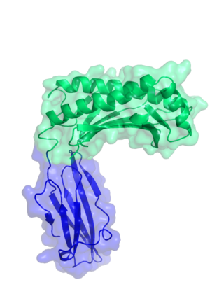
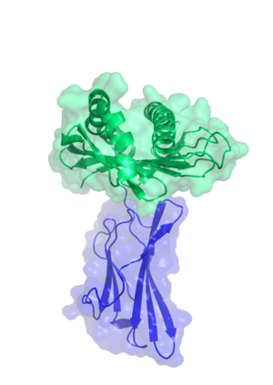
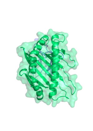
<xr id="corr_motions"/> shows two distinct zones with correlated movement. The first zone starts at the beginning of the sequence and ends at residue 175. The second zone starts at residue 176 and extends until the end of the sequence. Based on this observation, two domains can be assigned to the two zones. SCOP, CATH and Pfam all assign the same two domains to the HFE protein. <xr id="1a6z_domains" /> shows a 3D visualisation of the HFE protein and the MHC I domain (green) and the immunoglobulin domain (blue). This is in complete accordance with the domain assignment based on the correlated motion matrix.
References:
CATH MHC domain CATH Ig domain
SCOP MHC domain SCOP Ig domain
<figure id="1a6z_domains">
</figure>
Flexibility
<figure id="fluctuations">
</figure>
The HFE protein contains regions that are more flexible than others. <xr id="fluctuations"/> contains a plot from webNMA that shows for each residue on the x-axis the normalized squared fluctuations. High peaks correspond to highly flexible regions, which are connected by rigid stretches.
<figure id="3d_fluc">
</figure>
Another way to look at the C-alpha fluctuation data is shown in figure <xr id="3d_fluc"/>. The more flexible regions are almost exclusively located at the ends of the protein, that are farthest away from the hinge, that is the stretch, that connects the two domains.
Comparison of Molecular Dynamics and Normal Mode Analysis
In comparison to Molecular Dynamics, normal mode analysis can grasp the slow and globular motions of a protein. Although it can only grasp the harmonic part of these motions, it gives a good insight into them at comparably low computational cost. MD takes the influence of the side chains into account by modeling them explicitly, whereas NMA only takes them into account implicitly through the position of the C-alphas. Thus, MD can model the effect of side chain movements and SNPs on the proteins dynamics, whereas NMA cannot do this.
References
<references />


