Structure-based mutation analysis (Phenylketonuria)
Page still under construction!!!
Contents
Summary
In Task 8 the sequence of PAH was used for finding mutational effects, now the structure will be taken for these analysis. But how to find out, if a mutation changes the structure? Therefore, one calculates the energy of all atoms for the wildtype and the mutated structure and compares the results for changes. There are two different methods for this calculations given: Quantum Mechanics (QM) and Molecular Mechanics (MM). In QM the energy of all electrons in a protein is calculated. It is one of the most accurated methods, but it is very time consuming. In MM the energy of a system is calculated as a function of nuclear positions. It is very fast and easy to calculate, but it ignores electronic motions and is not as accurate as QM. Since QM is too time intensive and the results of MM are nearly as good as the ones calculated with QM, we use MM for the further analysis. Molecular Mechanics uses force fields for the energy calculation, which is defined as a sum of terms. The terms are non-bonded (electrostatic and Van-der-Waals) and bonded (Bond stretching, Angle stretching, bond rotation) interactions. For the structure based mutation analysis the tools SCWRL and FoldX were used.
Structure selection
In some Tasks before, we used the protein structure of 2PAH as reference, but now we have to check some more constraints for the protein structure selection:
- Structure with the highest resolution (small Å value),
- smallest R-factor,
- highest coverage,
- pH-value ideally near physiological pH of 7.4 and
- no gaps (missing residues) included in the structure, so a consecutive numbering of residues should be given.
To check which protein structure to use for further analysis, we compared the constraint data for all sequences given in the PAH (P00439) Uniprot entry. <figtable id="pro-struc">
| Protein | Method | Resolution(Å) | R-factor | pH | Gaps | Chain | Positions | Coverage % |
|---|---|---|---|---|---|---|---|---|
| 1DMW | X-ray | 2.00 | 0.20 | 6.80 | - | A | 118-424 | 67,92 |
| 1J8T | X-ray | 1.70 | 0.20 | 6.80 | - | A | 103-427 | 71.90 |
| 1J8U | X-ray | 1.50 | 0.16 | 6.80 | - | A | 103-427 | 71.90 |
| 1KW0 | X-ray | 2.50 | 0.22 | 6.80 | - | A | 103-427 | 71.90 |
| 1LRM | X-ray | 2.10 | 0.21 | 6.80 | - | A | 103-427 | 71.90 |
| 1MMK | X-ray | 2.00 | 0.20 | 6.80 | - | A | 103-427 | 71.90 |
| 1MMT | X-ray | 2.00 | 0.21 | 6.80 | - | A | 103-427 | 71.90 |
| 1PAH | X-ray | 2.00 | 0.18 | 6.80 | - | A | 117-424 | 68.14 |
| 1TDW | X-ray | 2.10 | 0.21 | 6.80 | - | A | 117-424 | 68.14 |
| 1TG2 | X-ray | 2.20 | 0.21 | 6.80 | - | A | 117-424 | 68.14 |
| 2PAH | X-ray | 3.10 | 0.25 | 7.00 | 136LEU-143ASP | A/B | 118-452 | 74.12 |
| 3PAH | X-ray | 2.00 | 0.18 | 6.80 | - | A | 117-424 | 68.14 |
| 1ANP | X-ray | 2.11 | 0.20 | 6.80 | - | A | 104-427 | 71.68 |
| 4PAH | X-ray | 2.00 | 0.17 | 6.80 | - | A | 117-424 | 68.14 |
| 5PAH | X-ray | 2.10 | 0.16 | 6.80 | - | A | 117-424 | 68.14 |
| 6PAH | X-ray | 2.15 | 0.17 | 6.80 | - | A | 117-424 | 68.14 |
</figtable> All structures do not cover the whole PAH protein and were found with the X-ray diffraction method. In <xr id="pro-struc"/> we can see, that the structure of 1J8U has a better resolution value as well as R-factor than the other structures. Although 2PAH has a better pH-value, a higher coverage and even two chains, however, the structure includes one gap. For this reason as well as the better R-factor and higher resolution value, we have chosen the structure of 1J8U for further analysis. 1J8U is the catalytic domain of human phenylalanine hydroxylase Fe(II) and does not contain any gaps. Moreover, the structure includes the second highest coverage and also a very good pH-value.
The 3D structure of 1J8U as well as its ligands are shown in the <xr id="1j8u"/> below. The binding site for the ligand FE(II) consists of the residues His285, His290 and Glu330 and the one for ligand H4B consists of Val245, Gly247, Leu249 and Ser251. Both were taken from the pdb entry of 1J8U. These binding sites are shown in detail in <xr id="bindingsite"/>.
</figure> </figure>| <figure id="1j8u"> |
| <figure id="bindingsite"> |
Visualisation of used mutations
Following five mutations from the previously selected mutations in Task8 are mapped to the crystal structure:
| Substitution | Prediction | Database |
|---|---|---|
| Gln172His | neutral | dbSNP |
| Ala259Val | non-neutral | HGMD |
| Thr266Ala | non-neutral | dbSNP |
| Phe392Ser | non-neutral | dbSNP |
| Pro416Gln | non-neutral | HGMD |
For the conversion of the residues, which include a mutation, we used the Mutagenesis tool in PyMOL. A little overview of the mutations is located in the next subsections with associated figures.
Gln172His
<figure id="Q172H">
</figure>
This mutation is located far away from any of the binding sites, so one would not expect a huge effect on the protein.
Ala259Val
<figure id="A259V">
</figure>
...
Thr266Ala
<figure id="T266A">
</figure>
In <xr id="T266A"/> we can see, that this residue is not located directly to the binding sites, but it lies between both ones. So, we would expect, that this mutation is disease causing.
Phe392Ser
<figure id="F392S">
</figure>
Since this mutations lies far away from both binding sites, we would expect only a small effect on the protein.
Pro416Gln
<figure id="P416Q">
</figure>
...
Mutated structure creation
SCWRL4
SCWRL4 (Side-chain Conformation Prediction With Rotamer Library) predicts protein side-chain conformations. Therefore, it uses a backbone-dependent rotamer library. The tool is based on graph theory, easy to use, accurate and very fast. The output includes a 3D structure of the prediction. <ref name="scwrl4"> Georgii G. Krivov1, Maxim V. Shapovalov1 and Roland L. Dunbrack Jr. (2009): "Improved prediction of protein side-chain conformations with SCWRL4". Proteins Vol.77(4):778-95. doi:10.1002/prot.22488</ref> There is also an online SCWRL Server available.
After generating the mutated structures with SCWRL, we compared the results to the wildtype structure in Pymol and checked if only the mutated side chain or another one has been changed. In the observation, only the mutated side chain was changed.
...
FoldX
FoldX ...
<figtable id="foldx">
| Type | Total energy | Backbone Hbond | Sidechain Hbond | Van der Waals | Electrostatics | Solvation Polar | Solvation Hydrophobic | Van der Waals clashes | Entropy sidechain | Entropy mainchain | Sloop entropy | Mloop entropy | Cis bond | Torsional clash | Backbone clash | Helix dipole | Water bridge | Disulfide | Electrostatic kon | Partial covalent bonds | Energy Ionisation | Entropy Complex |
|---|---|---|---|---|---|---|---|---|---|---|---|---|---|---|---|---|---|---|---|---|---|---|
| WT | x | x | x | x | x | x | x | x | x | x | x | x | x | x | x | x | x | x | x | x | x | x |
| Q172H | 13.84 | -196.19 | -56.45 | -378.50 | -19.95 | 492.48 | -495.07 | 33.39 | 193.60 | 453.85 | 0.00 | 0.00 | 0.00 | 11.68 | 227.36 | -14.78 | -11.79 | 0.00 | 0.00 | 0.00 | 1.55 | 0.00 |
| A259V | 14.08 | -198.14 | -59.00 | -379.98 | -19.12 | 495.02 | -497.16 | 34.93 | 194.60 | 454.17 | 0.00 | 0.00 | 0.00 | 13.19 | 227.82 | -15.57 | -10.30 | 0.00 | 0.00 | 0.00 | 1.45 | 0.00 |
| T266A | 15.08 | -196.56 | -56.37 | -378.45 | -19.86 | 493.23 | -494.94 | 32.68 | 193.42 | 453.13 | 0.00 | 0.00 | 0.00 | 11.94 | 227.53 | -15.13 | -9.46 | 0.00 | 0.00 | 0.00 | 1.45 | 0.00 |
| F392S | 24.59 | -195.99 | -57.60 | -377.49 | -19.29 | 495.41 | -492.28 | 34.80 | 193.85 | 453.89 | 0.00 | 0.00 | 0.00 | 11.71 | 227.42 | -15.39 | -8.47 | 0.00 | 0.00 | 0.00 | 1.45 | 0.00 |
| P416Q | 21.20 | -196.09 | -57.10 | -379.58 | -19.53 | 496.13 | -495.90 34.25 | 195.06 | 454.65 | 0.00 | 0.00 | 0.00 | 11.44 | 228.58 | -15.11 | -8.47 | 0.00 | 0.00 | 0.00 | 1.45 | 0.00 |
... </figtable>
Comparison
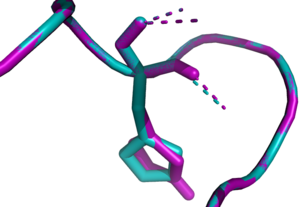
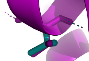
Now, we want to compare the results of SCWRL and FoldX. Therefore, we loaded the pdb structures into PyMOL and looked after differences between the two results. There was only one change in the 3D structure of the two programs, which can be seen in figure x.
</figure> </figure>| <figure id="comparison_all"> |
| <figure id="comparison_part"> |
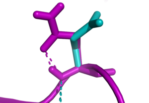
We also compared the two structures with the wildtype 1J8U structure and there are some little changes, but the interesting part was the change between SCWRL and FoldX. FoldX has the beta strand on the position of the wildtype structure whereas the one of SCWRL has changed. Since it is only a small difference in the structures, we do not think, that it has a huge consequence for the protein.
It is also very interesting, which changes the SCWRL and FoldX outputs show in each mutation. Hence, we want to analyse every mutation on its own.
</figure> </figure> </figure> </figure> </figure>
| <figure id="comparison_Q172H"> |
| <figure id="comparison_A259V"> |
| <figure id="comparison_T266A"> |
| <figure id="comparison_F392S"> |
| <figure id="comparison_P416Q"> |
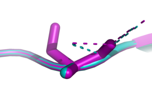
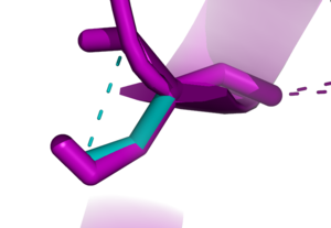
All in all one can see, that SCWRL has hydrogen atoms in the structures included, which FoldX does not. Furthermore, do all mutations got a slight twisting. But in the whole, there are only small changes between the two tools.
Energy comparisons
<figtable id="scwrl">
| SCWRL results | |||
|---|---|---|---|
| Type | Energy | Energy Mutation / Energy Wildtype |
Prediction |
| WT | 164.210 | 1.00 | - |
| Q172H | 169.699 | 1.03 | x |
| A259V | 197.235 | 1.20 | x |
| T266A | 167.116 | 1.02 | x |
| F392S | 171.409 | 1.04 | x |
| P416Q | 169.007 | 1.03 | x |
Comparison of the SCWRL results between the wildtype and the mutant structures. In the first column the type (mutation or wildtype) is given, then the resulting total minimal energy of the graph from the SCWRL results. In the third column this energy is divided through the wildtype resulting energy, to check the difference between this two types, and in the last column the prediction of the SCWRL results is represented. </figtable> ...
Minimise
In the table below, the energy for all five runs of minimise are given. Since the SCWRL output could not be minimised, we only can see the difference between the wildtype (WT) and the five mutation structures constructed with foldX. <figtable id="minimise">
| minimise run | |||||
|---|---|---|---|---|---|
| Type | 1 | 2 | 3 | 4 | 5 |
| WT | -7516.27 | -7524.20 | -7291.36 | -7133.71 | -6996.34 |
| Q172H | -7514.27 | -7504.92 | -7281.60 | -7131.31 | -7023.56 |
| A259V | -7469.61 | -7462.48 | -7221.58 | -7065.94 | -6951.32 |
| T266A | -7536.77 | -7523.38 | -7298.14 | -7165.29 | -7084.60 |
| F392S | -7511.51 | -7528.61 | -7290.01 | -7132.75 | -7010.52 |
| P416Q | -7556.57 | -7542.79 | -7299.39 | -7151.21 | -7040.37 |
</figtable> The energies of the wildtype and the mutated structures is very similar and is per run increasing slightly. Only for the structures of the wildtype and the mutation F392S has the second run a small decreased value.
References
<references/>


