Fabry:Molecular Dynamics Simulations Analysis
Fabry Disease » Molecular Dynamics Simulations Analysis
Contents
Thermodynamics
In the following we compared the temperature, pressure, potential energy and total energy development in the wildtype and the three mutants over time.
Temperature
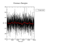
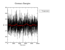
In all four simulations the temperature fluctuates around the reference of 298K and maximaly changes by 3 degrees. There seem to be no significant differences between the wildtype and the mutants.
<figtable id="tab:temperature"> This table shows the time course of the temperature in the MD analysis of the wildtype and the mutants in black. The average temperature value over 100 steps, which refers to 500ps, is denoted in red.
</figtable>
Pressure
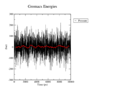
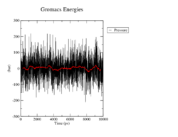
The average pressure again does not differ a lot from the specified 1 bar, although the pressure fluctuates by up to 300. Again, we cannot observe large differences between the mutants and the wildtype.
<figtable id="tab:pressure"> This table shows the time course of the pressure in the MD analysis of the wildtype and the mutants in black. The average pressure value over 100 steps, which refers to 500ps, is denoted in red.
</figtable>
Potential and total energy
There is a small decline in the average potential energy (see <xr id="tab:potential"/>) of all four molecules, since the respective structure is optimised during the simulations. This results in an average potential energy of about -167600 kJ/mol for all simulations, with a slightly higher average in the R356W mutant. We can also see a decline in the average total energy (see <xr id="tab:total"/>) to about -137500 kJ/mol in all four simulations.
<figtable id="tab:potential"> This table shows the time course of the potential energy in the MD analysis of the wildtype and the mutants in black. The average potential energy value over 100 steps, which refers to 500ps, is denoted in red.
</figtable>
<figtable id="tab:total"> This table shows the time course of the total energy in the MD analysis of the wildtype and the mutants in black. The average total energy value over 100 steps, which refers to 500ps, is denoted in red.
</figtable>
Minimum distance between periodic images
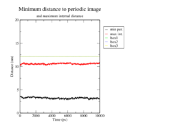
To prevent unphysical interactions with a copy of the molecule itself in an adjacent box, the minimum distance of periodic images should not fall below 2 nm. As we can see, this does not happen in any of the four cases. The distances stay fairly constant around 3 nm over the whole simulation, without any large outliers.
<figtable id="tab:minDist"> This table shows the minimum distance of periodic images in the MD analysis of the wildtype and the mutants in black.
</figtable>
Root mean square fluctuations
<figure id="fig:Palette">

</figure>
<figure id="fig:actSite">

</figure>
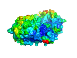
As one can see in the Figure A of <xr id="tab:RMSD"/>, the fluctuation in the wildtype molecule range from low (blue) to medium-high (yellow) in most parts of the molecule, except for four loops on the outside, that are very flexible (orange and red color). The outer part of the "large" region of each monomere and the linking parts are more flexible than the "small" regions of the monomeres. This effect is reversed in the I289V mutant (see <xr id="tab:RMSD"/>, Fig B), where the large part is rigid (almost completely colored) blue and the small part is not. Comparing this observation to the figures E and F in <xr id="tab:RMSD"/>, we can see that in fact the first 100 amino acids in the mutant have a higher RMSF than the wildtype, but the middle part (residue 140 - 300) has less fluctuation. Even less flexible is the mutant R118H, where we can observe no large fluctuation except for the loop that is formed by the end of the sequence (see <xr id="tab:RMSD"/>, Fig D and H). The least RMS fluctuations can be observed in the R356W mutant (see <xr id="tab:RMSD"/>, Fig C and G), where there are only two flexible regions, one in the beginning of the sequence and one in the end. The binding region that is formed by the residues 203 - 207 seems to be especially rigid in this mutant, which may be an indicator for the disease causing nature of this protein (see also <xr id="fig:actSite"/>). The active site's fluctuation is only little reduced in the other mutants, which is an indicator for the non-disease causing nature of them.
<figtable id="tab:RMSD"> This table shows the residue-wise B-Factor of the four molecules, where red represents great movement and blue a rather rigid structure (see <xr id="fig:Palette"/>), as well as the corresponding root mean square fluctuations plots.
</figtable>
Radius of gyration
There are almost no differences in the radii of gyration among the four simulations as we can see in <xr id="tab:gyration"/>. This number represents the overall shape of the molecule, which aparently did not change due to the mutations or during the simulations.
<figtable id="tab:gyration"> This table shows the radii of gyration of the wildtype's and the three mutant's simulations.
</figtable>
RMSD
The root mean square deviation of the structures first of all is compared to the RMSD of the average of all structures (see <xr id="tab:rmsd"/>, Fig. A-D). We can see that all simulations in the beginning more or less fast converged towards a structure with a mean RMSD of about 0.15. In the case of the wildtype protein the RMSD again jumps back to its starting mean of approximately 0.25. From this we could conclude that the molecule structure again posseses its starting structure, but this theory is not supported by the comparison of the RMSD of the structures in the end with the starting structure's (see <xr id="tab:rmsd"/>, Fig. E). The RMSD constantly rises over time, making it impossible that the starting and the end structure are the same. As expected, the comparison to the mutant's starting structures is also monotonic increasing.
For all four molecules only little change in clustering can be observed, indicated by the few red color in <xr id="tab:rmsd"/>, Fig. I-L.
<figtable id="tab:rmsd"> This table shows different root mean square deviations of the wildtype and the three mutants compared to different structures.
</figtable>
Hydrogen bonds
As depicted in <xr id="tab:hbonds"/>, Fig. A-D, there is hardly any difference in the time courses of the number of hydrogen bonds within the mutants compared to the wildtype. The number fluctuates around 600 in all four molecules, without any larger deviations. There is little difference in the number of hydrogen bonds to the solvent (<xr id="tab:hbonds"/>, Fig. E-H). In the time course of the wildtype we can see a steep increase in the first thousand time steps and then again a decrease that moves towards the mean of 1400 hydrogen bonds to water (see Fig. E). The behaviour of the mutant R356W (Fig. G) looks similar. The mutants I289V and R118H show a different time course. There is a less steep increase of the number of hydrogen bonds until a maximum is reached, this level is held until the end of the simulation.
<figtable id="tab:hbonds"> This table shows the time course of the number of hydrogen bonds within the wildtype and the three mutants (A-D), as well as the number of hydrogen bonds of each molecule to the surrounding water (E-H)
</figtable>
References
<references/>
