Task 10: Molecular Dynamics Analysis

In this task we are going to analyze the results of the molecular dynamics simulations of task 8. A detailed task description can be found here. The analysis focuses on this tutorial.

Native

A BRIEF CHECK OF RESULTS

In order to verify that our simulation ran successfully we used the command line tool gmxcheck. we executed it as follows for our .xtc file:

gmxcheck -f 1J8U_nosol_after_SCWRL_no_h_merged_crystal_water_md.xtc

How many frames are in the trajectory file and what is the time resolution?

We observed 2001 frames with a time resolution of 5ps.

How long did the simulation run in real time (hours), what was the simulation speed (ns/day) and how many years would the simulation take to reach a second?

The simulation ran 4h00:39 and had a simulation speed of 59.835 ns/day. To calculate 1 second we would need (1 / (59 * (10^(-9)))) / 365 = 46 436.0344 years

Which contribution to the potential energy accounts for most of the calculations?

• potential energy: -4.57312e+05 kJ/mol

VISUALIZATION OF RESULTS

We extracted 1000 frames from the trajectory (-dt 10), leaving out the water (selected Protein when asked for a selection). Moreover, we will remove the jumps over the boundaries and make a continuous trajectory (-pbc nojump):

trjconv -s 1J8U_nosol_after_SCWRL_no_h_merged_crystal_water_md.tpr -f 1J8U_nosol_after_SCWRL_no_h_merged_crystal_water_md.xtc -o protein.pdb -pbc nojump -dt 10

After that we opened the generated protein.pdb file with pymol. Here we changed the coloring to spectrum by typing the following to the pymol command line:

spectrum

In a next step we enabled the the visualization of the cell with this command:

show cell

In order to remove the tumbeling and wiggeling motion of our protein we used the command intra_fit since we are only interested in the internal motions of the protein:

intra_fit protein

The results of these actions can be seen in figure 1 and 2. Figure one shows our WT protein in line view which makes it able to see the motion of the side chains. Figure to shows the protein in cartoon view to see the overall movement of the secondary structure elements.

Figure 1: motion of protein in line view

Figure 2: motion of protein in cartoon view

QUALITY ASSURANCE

CONVERGENCE OF ENERGY TERMS

In this part of quality assurance we analyzed different metrics of our MD simulation by creating plots from our *.edr file. We created plots for the temperature, pressure, energy, volume, density, box, coulomb and van der waals values of our MD simulation by using the tool g_energy as follows:

//calculating temperature enter then "12 0" 
g_energy -f 1J8U_nosol_after_SCWRL_no_h_merged_crystal_water_md.edr -o ../../../Dropbox/Studium/3_semester/master_praktikum/task10/temperature.xvg

//calculating pressure enter then "13 0" 
g_energy -f 1J8U_nosol_after_SCWRL_no_h_merged_crystal_water_md.edr -o ../../../Dropbox/Studium/3_semester/master_praktikum/task10/pressure.xvg

//calculating energy (potential, kinetic and total) enter then "9\n10\n11 0" 
g_energy -f 1J8U_nosol_after_SCWRL_no_h_merged_crystal_water_md.edr -o ../../../Dropbox/Studium/3_semester/master_praktikum/task10/energy.xvg

//calculating volume enter then "18 0" 
g_energy -f 1J8U_nosol_after_SCWRL_no_h_merged_crystal_water_md.edr -o ../../../Dropbox/Studium/3_semester/master_praktikum/task10/volume.xvg

//calculating density enter then "19 0" 
g_energy -f 1J8U_nosol_after_SCWRL_no_h_merged_crystal_water_md.edr -o ../../../Dropbox/Studium/3_semester/master_praktikum/task10/density.xvg

//calculating box enter then "15\n16\n17 0" 
g_energy -f 1J8U_nosol_after_SCWRL_no_h_merged_crystal_water_md.edr -o ../../../Dropbox/Studium/3_semester/master_praktikum/task10/box.xvg

//calculating coulomb enter then "48\n50 0"
g_energy -f 1J8U_nosol_after_SCWRL_no_h_merged_crystal_water_md.edr -o ../../../Dropbox/Studium/3_semester/master_praktikum/task10/coulomb-inter.xvg

//calculating van der waals enter then "49\n51 0"
g_energy -f 1J8U_nosol_after_SCWRL_no_h_merged_crystal_water_md.edr -o ../../../Dropbox/Studium/3_semester/master_praktikum/task10/vanderwaals-inter.xvg

Temperature Over Time

Figure 3: Fluctuation of temperature over time in WT

"Energy"	"Average"	"Err.Est."	"RMSD"	"Tot-Drift"
"Temperature"	297.886	0.007	1.57824	"-0.0105059 (K)"

In figure 3 we can see that the temperature stays quite the same over the whole simulation which might be interpreted as that our system has reached its stable temperature for simulation.

Pressure over Time

Figure 4: Fluctuation of pressure over time in WT

"Energy"	"Average"	"Err.Est."	"RMSD"	"Tot-Drift"
"Pressure"	1.02313	0.023	133.659	"-0.0928554 (bar)"

Energy over Time

Figure 5: Potential, kinetic and total energy over time in WT

"Energy"	"Average"	"Err.Est."	"RMSD"	"Tot-Drift"
"Potential"	-457312	61	640.502	" -423.792 (kJ/mol)"
"Kinetic En."	81855.1	1.9	433.677	" -2.88684 (kJ/mol)"
"Total Energy"	-375457	61	784.246	" -426.678 (kJ/mol)"

Volume over Time

Figure 6: Fluctuation of volume over time in WT

"Energy"	"Average"	"Err.Est."	"RMSD"	"Tot-Drift"
"Volume"	356.629	0.041	0.397685	" -0.151337 (nm^3)"

Density over Time

Figure 7: Fluctuation of density over time in WT

"Energy"	"Average"	"Err.Est."	"RMSD"	"Tot-Drift"
"Density"	1021.28	0.12	1.13884	"0.433467 (kg/m^3)"

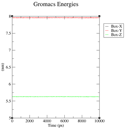
Box over Time

Figure 8: box size over time in WT

"Energy"	"Average"	"Err.Est."	"RMSD"	"Tot-Drift"
"Box-X"	7.95996	" 0.0003"	0.00295875	"-0.00112603 (nm)"
"Box-Y"	7.95996	" 0.0003"	0.00295875	"-0.00112603 (nm)"
"Box-Z"	5.62854	0.00021	0.00209216	"-0.000796226 (nm)"

Coulomb over Time

Figure 9: Fluctuation of coulomb energies over time in WT

"Energy"	"Average"	"Err.Est."	"RMSD"	"Tot-Drift"
"Coul-SR:Protein-non-Protein"	" -20429.9"	"110"	"425.888"	"-561.713 (kJ/mol)"
"Coul-14:Protein-non-Protein"	" 0"	" 0"	" 0"	" 0 (kJ/mol)"

Van der Waals over Time

Figure 10: Fluctuation of van der waals energies over time in WT

"Energy"	"Average"	"Err.Est."	"RMSD"	"Tot-Drift"
"LJ-SR:Protein-non-Protein"	"-2172.28"	"15"	"136.956"	"-103.12 (kJ/mol)"
"LJ-14:Protein-non-Protein"	" 0"	" 0"	" 0"	" 0 (kJ/mol)"

Questions

1. What is the average temperature and what is the heat capacity of the system?

The average temperature of our system is 297.886 K and the heat capacity ranges from 303 to 292. (values taken from figure 3).

2. What are the terms plotted in the files energy.xvg and box.xvg

3. Estimate the plateau values for the pressure, the volume and the density.

4. What are the terms plotted in the files coulomb-inter.xvg and vanderwaals-inter.xvg