Difference between revisions of "Molecular Dynamics Simulations Analysis Gaucher Disease"
(→Analysis of dynamics and time-averaged properties) |
|||
| Line 290: | Line 290: | ||
== Analysis of dynamics and time-averaged properties == |
== Analysis of dynamics and time-averaged properties == |
||
| + | For checking the existence of particular conformations which often recurs in the MD simulation, we clustered all structures in the trajectory. The root mean square deviation (RMSD) was used for measuring the distance of two structures. All backbone atoms and the C-beta atom was taking into account for computing the RMSD. Next, an iterative clustering algorithm was employed which determines in each iteration the number of neighbors of all structures and determines the structure with the highest number of neighbors. Next, it clusters this structures and all its neighbors and proceeds with all remaining structures. Neighbors are all structures with a RMSD below user defined cut-off value. We chose 0.9 as cut-off for obtaining more than 10 clusters. |
||
| + | |||
| + | <xr id="fig:cluster_clusters"/> depicts the RMSD between all structures in the trajectory and whether they belong to the same cluster. <xr id="fig:cluster_time"/> shows to which cluster structures in the trajectory belong to where the clusters are sorted by the number of cluster members. A superposition of the two largest clusters is shown in <xr id="fig:cluster_super"/>. |
||
| + | |||
For quantifying the similarity of structures in the trajectory, we computed the Root Mean Square Deviations (RMSD) between all structures in the trajectory. Both for least-square fitting and for calculating the RMSD, the backbone and the C-beta atom was taken into account. |
For quantifying the similarity of structures in the trajectory, we computed the Root Mean Square Deviations (RMSD) between all structures in the trajectory. Both for least-square fitting and for calculating the RMSD, the backbone and the C-beta atom was taken into account. |
||
| Line 300: | Line 304: | ||
<small><caption>Upper half:RMSD between all pairs of structures in the trajectory. Lower half: Red and blue dots correspond to pairs of structures belonging to the same and different cluster, respectively.</caption></small> |
<small><caption>Upper half:RMSD between all pairs of structures in the trajectory. Lower half: Red and blue dots correspond to pairs of structures belonging to the same and different cluster, respectively.</caption></small> |
||
</figure> |
</figure> |
||
| − | |||
<figure id="fig:cluster_time"> |
<figure id="fig:cluster_time"> |
||
| Line 320: | Line 323: | ||
</figure> |
</figure> |
||
| + | === Wildtype === |
||
| + | There are three major clusters in the wildtype trajectory with 685 (cluster 1), 163 (cluster 2), and 69 (cluster 3) structures. The majority of structures up to a simulation time of 2000ps belong to cluster 2. At 2000ps, there is a transition from cluster 2 to cluster 1 which covers most structures until the end of the simulation. In other words, the conformation changes conspicuously at 2000ps and then remains stable until 10ns expect for some transition to a conformation described by cluster 3. Cluster 2 and cluster 1 mainly differ in loop regions of the hydrolase domain (<xr id="fig:cluster_super#1"/>) |
||
=== Distance RMSD === |
=== Distance RMSD === |
||
Revision as of 00:35, 13 August 2012
In this task, we followed the steps of the molecular modeling practical by the University Utrecht[1] for analysing the molecular dynamics simulations which were set up in Task 8. After we had verified that the MD simulations terminated properly, we employed tools of the GROMACS package<ref name="gromacs">Erik Lindahl, Berk Hess, and David van der Spoel. GROMACS 3.0: a package for molecular simulation and trajectory analysis. Journal of Molecular Modeling, 7(8):306–317, August 2001.</ref> to investigate the dynamics of GCase (2nt0_A) and the mutants L470P as well as W209. Technical details can be found in our protocol.
Contents
A brief check of results
We briefly checked the length of the MD simulations via gmxcheck. Since we used the AGroS paramter -lengthMD 10, we expected the MD simulation to be 10 ns long. gmxcheck reported for each simulation 2001 frames and a time step of 5 ps per frame which amounts to the expected length of 2001*5ps=10ns.
We further investigated the runtime of the MD simulation by looking at the log files. The simulation of the WT took approximately twice as long as the other two mutations since we used only 16 instead of 32 cores. Performing a MD simulation over 1s would take more than 100000 years if the same hardware were used than we did.
<figtable id="tab:runtime">
| Name | Runtime | ns/day | years/1s | |
|---|---|---|---|---|
| WT | 16h25:59 | 14.605 | 187536 | |
| L470P | 9h20:49 | 25.677 | 106699 | |
| W209R | 9h18:47 | 25.770 | 106314 | |
Runtime of the MD simulations and the estimated runtime for a simulation length of 1s. </figtable> The computation of the energy term Coul(T) + LJ [W3-W3] accounted for most (47%) of the floating point operations.
Visualization
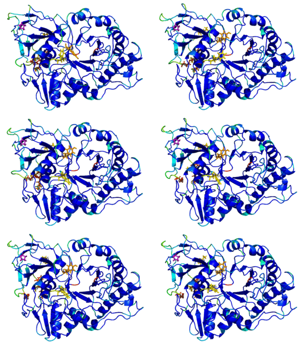
For getting a first impression of the MD simulations, we visualized the structures stored in the trajectory files. A course grained animation of the three simulations with 29 frames is shown in <xr id="fig:viz"/>. Altogether, the animations indicate that all three simulations terminated successfully without sever structural changes. Based on the visual inspection, we could not detect any rearrangements which would suggest a malign effect of one of the mutations. However, the active site residue E235 and E340 might be more flexible in L470P compared to the wildtype.
<figure id="fig:viz">
</subfigure> </subfigure> </subfigure>| <subfigure> |
| <subfigure> |
| <subfigure> |
Visualization of the MD simulations. Red: the active site residues E235 and E340; Blue: the mutated residue. </figure>
Quality assurance
We checked the quality of the MD simulations regarding the convergence of the pressure, temperature, potential energy, and total energy. Strongly fluctuating thermodynamic parameters and insufficiently converging parameters might hint at problems during the MD simulations or a lacking equilibration.
<xr id="fig:qual_pres"/> shows the development of the pressure along the MD simulations. In all three cases, the pressure fluctuates between -200 and 200 bar but the average pressure of 1 bar does not change. In contrast the the wildtype which exhibits a negative drift, the pressure slightly increases in case of L470P and W209R.
<figure id="fig:qual_pres">
</subfigure> </subfigure> </subfigure>| <subfigure> |
| <subfigure> |
| <subfigure> |
Development of the pressure during the MD simulation. In brackets: average/total-drift. </figure>
The temperature of 297.9 K remains constant and varies by only +/- 2 K (<xr id="fig:qual_temp"/>).
<figure id="fig:qual_temp">
</subfigure> </subfigure> </subfigure>| <subfigure> |
| <subfigure> |
| <subfigure> |
Development of the temperature during the MD simulation. In brackets: average/total-drift. </figure>
Both the potential energy and the total energy reduces at the beginning of the MD simulations (<xr id="fig:qual_pot"/>, <xr id="fig:qual_tot"/>). L470P shows the strongest shift towards the negative range, i.e. the stability of the structure increases most.
<figure id="fig:qual_pot">
</subfigure> </subfigure> </subfigure>| <subfigure> |
| <subfigure> |
| <subfigure> |
Development of the potential energy during the MD simulation. In brackets: average/total-drift. </figure>
<figure id="fig:qual_tot">
</subfigure> </subfigure> </subfigure>| <subfigure> |
| <subfigure> |
| <subfigure> |
Development of the total energy during the MD simulation. In brackets: average/total-drift. </figure>
Self-interactions between periodic images are unphysical and might disturb the MD simulations. We therefore checked the minimal distance to adjacent cells by taking (a) only C-alpha atoms and (b) also side-chain atoms into account (<xr id="fig:mindist"/>).
In all three simulations, the minimal distance slightly decreases but does not falls below the cut-off distance of 2 nm. If only C-alpha atoms are taking into account, the minimal distance is bout 0.5 nm higher compared to using all protein atoms. This corresponds to an average side-chain length of 5 A. For W209R, the minimal distance drops below 2 nm at 9180 ps but then increases again such that this event does not impact the MD simulation.
<figure id="fig:mindist">
</subfigure> </subfigure> </subfigure>| <subfigure> |
| <subfigure> |
| <subfigure> |
Minimal distance to the adjacent cell with respect C-alpha atoms (black) and all protein atoms (red). In brackets: time frame and minimal distance for c-alpha/protein atoms. </figure>
The radius of gyration (Rg) is the root mean square deviation of all atoms from the centroid or the main diagonals of the protein. It is therefore used to quantify the overall shape of the protein. <xr id="fig:gyrate"/> depicts the Rg of GCase for all three mutations which hardly changes. Hence, the protein conformations remained stable. <figure id="fig:gyrate">
</subfigure> </subfigure> </subfigure>| <subfigure> |
| <subfigure> |
| <subfigure> |
Raduis of gyration (Rg) of GCase during the simulated time frame. Black: Rg centroid; Red: Rg x-axis; Green: Rg y-axis; Blue: Rg z-axis. </figure>
<figure id="fig:rmsd_b_start">
</subfigure> </subfigure> </subfigure>| <subfigure> |
| <subfigure> |
| <subfigure> |
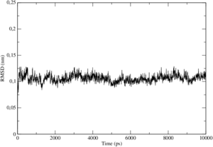
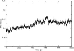
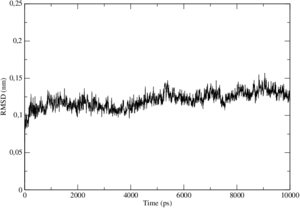
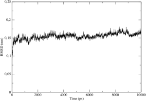
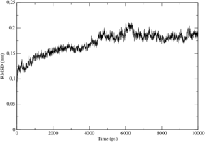
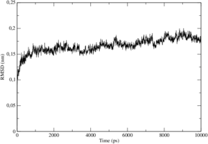
RMSD between backbone atoms of structures in the trajectory and the initial structure. </figure>
<figure id="fig:rmsd_p_start">
</subfigure> </subfigure> </subfigure>| <subfigure> |
| <subfigure> |
| <subfigure> |
RMSD between all protein atoms of structures in the trajectory and the initial structure. </figure>
<figure id="fig:rmsd_p_avg">
</subfigure> </subfigure> </subfigure>| <subfigure> |
| <subfigure> |
| <subfigure> |
RMSD between all protein atoms of structures in the trajectory and the average structure. </figure>
Flexibility
After we had verified that our MD simulations terminated probably, we investigated the flexibility of the wildtype and the mutant structures. We further compared the flexibility of L470P and W209R to the wildtype for identifying changes in the flexibility which might indicate perturbations of glycosylceramidase activity.
RMSF
For quantifying the flexibility we used the Root Mean Square Fluctation (RMSF). The RMSF of residue i is the mean square deviation from the position of i in the average structure. The average structures of all three simulations are shown in <xr id="fig:rmsf_avg"/> which were compared to the structure used for initializing the production run. Although the structures obviously changes during the simulation (<xr id="fig:viz"/>), the average structure hardly deviated from the initial structure in all three cases. Furthermore, we could not identify any significant changes between the average structure of the wildtype, L470P, and W209R.
<figure id="fig:rmsf_avg">
</subfigure> </subfigure> </subfigure>| <subfigure> |
| <subfigure> |
| <subfigure> |
Superposition of the average g_rmsf (green) structure onto the initial structure (blue). </figure>
<xr id="fig:rmsf_c"/> shows the RMSF of the C-alpha atoms which were used to color the residues in <xr id="fig:rmsf"/>. The fluctuation of all atoms per residue is depicted in <xr id="fig:rmsf_p"/>. The fluctuation patterns of <xr id="fig:rmsf_p"/> coincide with <xr id="fig:rmsf_c"/> but the amplitudes are more pronounced since side chains can rotate without changing the position of the C-alpha atom.
In all three simulations, the region 15-75 is fluctuating most which covers flexible loop regions of the hydrolase domain shown in the top left corner of <xr id="fig:rmsf"/>. Furthermore, the loop 341-350 at the center is moving dynamically, in particular residue F347 which belongs to the residues with the highest RMSF in all three simulations. The flexibility of loop 341-350 might be in fact functionally relevant since it is at the entrance of the TIM-beta/alpha-barrel domain which includes the active site residues E235 and E340. In W209R, the adjacent loop 393-396 is also fluctuating conspicuously.
<figure id="fig:rmsf">
</subfigure> </subfigure> </subfigure>| <subfigure> |
| <subfigure> |
| <subfigure> |
MD simulations with residues colored by the RMSF per residue and C-alpha atom. Red: high flexibility; Green: intermediate flexibility; Blue: low flexibility; Purple: mutant residue; Sticks: residues with the highest RMSF. </figure>
<figure id="fig:rmsf_c">
</subfigure> </subfigure> </subfigure>| <subfigure> |
| <subfigure> |
| <subfigure> |
RMSF per residue with respect to the C-alpha atom. </figure>
<figure id="fig:rmsf_p">
</subfigure> </subfigure> </subfigure>| <subfigure> |
| <subfigure> |
| <subfigure> |
RMSF per residue with respect to all atoms. </figure>
RMSF L470P vs. RMSF wildtype
For testing to which extent the motion of certain parts of L470P differ from the wildtype, we substracted the RMSF values of the wildtype from the RMSF values of L470P, i.e deltaRMSF = RMSFmut-RMSFwt. The difference of <xr id="fig:rmsf_c#2"/> and <xr id="fig:rmsf_c#1"/> is shown in <xr id="fig:rmsf_L470P_diff#1"/>: positive and negative values indicate regions in L470P which are more flexible and less flexible compared to the wildtype, respectively.
We further applied the two-sided Student's t-test for testing whether the mean of <xr id="fig:rmsf_L470P_diff#1"/> significantly deviates from zero, i.e. whether there is a significant difference in the fluctuation between the wildtype and L470P. For this, we first computed the test-statistic t=sqrt(n)*avg(deltaRMSF)/sd(deltaRMSF), where sqrt is the square root, avg the average, and sd the sampling standard deviation. Next, we computed the p-value P(|T| > t) using the t-distribution with n-1 degrees of freedom. And in deed, L470P is significantly (p-value 5e-13) more flexible compared to the wildtype.
In order to identify the regions which contribute most to the change in flexibility, we colored residues of L470P according to deltaRMSF. <xr id="fig:rmsf_L470P_diff#2"/> reveals that there are two loop regions (23-33, 42-53) underneath the hydrolase domain which are moving conspicuously. <xr id="fig:rmsf_L470P_diff#2"/> depicts that both loop regions are exposed and might be interacting with other constituents of the lysosomal membrane. These interactions might be disturbed by the increased flexibility due to L470P.
<figure id="fig:rmsf_L470P_diff">
</subfigure> </subfigure> </subfigure>| <subfigure> |
| <subfigure> |
| <subfigure> |
RMSF L470P compared to RMSF wildtype. The RMSF difference of Figure a were used for coloring residues. Red: higher flexibility; Green: same flexibility; Blue: lower flexibility; Purple: L470. Loop region 23-33 and 42-53 is significantly more flexible in L470P than in the wildtype. </figure>
RMSF W209R vs. RMSF wildtype
We investigated the difference of W209R and the wildtype in the same way as described above. <xr id="fig:rmsf_W209R_diff#1"/> illustrates that there are single residues whose mobility changed in W209R relative to the wildtype. Specifically, E395 (<xr id="fig:rmsf#3"/>) is more mobile, and T180 is less mobile. However, the overall fluctuation does not significantly (p-value 0.34) differ from the wildtype. We found that the positively charged mutant residue R209 forms a hydrogen bond to T180 (<xr id="fig:rmsf_W209R_diff#2"/>, <xr id="fig:rmsf_W209R_diff#3"/>) and therefore reduces the flexibility of T180. This might be one reason for the malign effect of W209R.
<figure id="fig:rmsf_W209R_diff">
</subfigure> </subfigure> </subfigure>| <subfigure> |
| <subfigure> |
| <subfigure> |
RMSF W209R compared to RMSF wildtype. The RMSF difference of Figure a were used for coloring residues. Red: higher flexibility; Green: same flexibility; Blue: lower flexibility; Purple: W209. The flexibility does not significantly differ from the wildtype. </figure>
Hydrogen bond network
Secondary structure elements like alpha-helices and beta-sheets are stabilised by hydrogen bonds between residues. Hence, changes in the hydrogen bond network can entail structural and functional changes. We therefore investigated the number of hydrogen bonds (HB) between protein residues (<xr id="fig:hbond_pp"/>) as well as between protein residues and water molecules (<xr id="fig:hbond_pw"/>).
The number of protein-protein HBs strongly fluctuates but remains constant for the wildtype and L470P. For W209R, the number decreases from 380 to about 370. There are on average 366 protein-protein HBs in case of L470P, significantly (two sample unpaired t-test) less compared to the wildtype.
The number of protein-water HBs is less robust then the number of protein-protein HBs, in particular for the wildtype (<xr id="fig:hbond_pw#1"/>) and W209R (<xr id="fig:hbond_pw#3"/>). In case of L470P, the number of HBs increases and converges to about 1300, significantly more compared to the wildtype.
In conclusion, L470P exhibits less HBs between residues and more HBs between residues and water molecules. This might account for higher flexibility described in #RMSF L470P vs. RMSF wildtype.
<figure id="fig:hbond_pp">
</subfigure> </subfigure> </subfigure>| <subfigure> |
| <subfigure> |
| <subfigure> |
Number of hydrogen bonds between protein residues along the MD simulation. The blue line indicates the mean number of hydrogen bonds. </figure>
<figure id="fig:hbond_pw">
</subfigure> </subfigure> </subfigure>| <subfigure> |
| <subfigure> |
| <subfigure> |
Number of hydrogen bonds between protein residues and water molecules along the MD simulation. The blue line indicates the mean number of hydrogen bonds. </figure>
Solvent Accessibility Surface
The solvent accessibility surface (SAS) of a residue is the area in angstrom^2 which is accessible for solvent molecules. It is further subdivided into the hydrophilic and hydrophobic SAS depending on which kind of interactions the residue area is accessible for. The ratio of the hydrophobic to hydrophilic SAS tends to be high for hydrophobic residues and low for hydrophilic residues. However, there are exception like lysine which exhibits the largest hydrophobic SAS due to its long carbon chain. Apart from physicochemical properties, the SAS of a residue also relies on the folding of a protein. The SAS per residue reduces on average by 20% as a result of folding and the total SAS of all residues is an indicator for the compactness of a protein. <ref name="sas">L. Lins, A. Thomas, and R. Brasseur. Analysis of accessible surface of residues in proteins. Protein Sci, 12(7):1406–1417, July 2003.</ref>
We therefore analysed the SAS of the three MD simulations (<xr id="fig:sas"/>). The hydrophobic SAS is smaller than the hydrophilic SAS suggesting that GCase has a hydrophobic core and is relatively compact. For the wildtype and W209R, the hydrophilic and hydrophobic SAS remains constant with about 122 and 102 nm^2, respectively. For L470P, the SAS increases along the MD simulation and is on average significantly higher compared to the wildtype using the unpaired two sample t-test.
<figure id="fig:sas">
</subfigure> </subfigure> </subfigure>| <subfigure> |
| <subfigure> |
| <subfigure> |
Size of total hydrophilic and hydrophobic SAS along the MD simulation. </figure>
SAS L470P vs. SAS Wildtype
By comparing the average SAS per residue of L470P to the wildtype, we indented to recognize structural changes caused by the mutation. For this, we computed the difference of the average SAS per residue for L470P and the wildtype, i.e. dSAS(i)=SAS_L470P(i)-SAS_WT(i). <xr id="fig:sas_L470P#1"/> depicts dSAS(i) for all residues i which were used to color the surface residues in <xr id="fig:sas_L470P#2"/>. F31 and M49, which belong to the loop regions described in #RMSF L470P vs. RMSF wildtype, are considerably more exposed in L470P compared to the wildtype. We conclude that L470P causes a reduction of inter protein hydrogen bonds which increases the flexibility of GCase and makes it more accessible for solvent molecules.
<figure id="fig:sas_L470P">
</subfigure> </subfigure>| <subfigure> |
| <subfigure> |
Size of SAS per residue of L470P compared to wildtype. SAS of F31 and M49 is enlarged. </figure>
SAS W209R vs. SAS Wildtype
The SAS of W209R does not change as much relative to the wildtype than L470P. dSAS is the lowest for Y313 (<xr id="fig:sas_W209R#1"/>) which is part of a beta-sheet close to the active site (<xr id="fig:sas_W209R#2"/>).
<figure id="fig:sas_W209R">
</subfigure> </subfigure>| <subfigure> |
| <subfigure> |
Size of SAS per residue of W209R compared to wildtype. SAS of Y313 is reduced. </figure>
Ramachandran plot
<figure id="fig:rama_gen">
</figure> The Ramachandran plot visualizes the dihedral angles phi and psi of amino acids of a protein structure (<xr id="fig:rama_gen"/>). Only phi/psi configurations which do not result in spatial clashed are allowed. These configurations depend on the side-chain of each residue and the secondary structure element they are part of. A Ramachandran plot can therefore shed light on the distribution of amino acids and the prevalence of secondary structure elements.
<xr id="fig:rama"/> depicts the Ramachandran plots for all three MD simulations. Each plot shows the phi/psi distribution of all 2001 structures in the trajectory and thus represents the average distribution of phi/psi angles. Alpha helices occur with the highest frequency and there are only few residues which do not belong to certain secondary structure regions. There are no remarkable differences between the Ramachandran plots of the three MD simulations which is consistent with the observation that that the structures keep a similar radius of gyration (<xr id="fig:gyrate"/>).
<figure id="fig:rama">
| <subfigure> |
| <subfigure> |
| <subfigure> |
Ramachandran plots showing the distribution of phi/psi angles of all 2001 structures in the trajectory. The coloring corresponds to the frequency of phi/psi. </figure>
Analysis of dynamics and time-averaged properties
For checking the existence of particular conformations which often recurs in the MD simulation, we clustered all structures in the trajectory. The root mean square deviation (RMSD) was used for measuring the distance of two structures. All backbone atoms and the C-beta atom was taking into account for computing the RMSD. Next, an iterative clustering algorithm was employed which determines in each iteration the number of neighbors of all structures and determines the structure with the highest number of neighbors. Next, it clusters this structures and all its neighbors and proceeds with all remaining structures. Neighbors are all structures with a RMSD below user defined cut-off value. We chose 0.9 as cut-off for obtaining more than 10 clusters.
<xr id="fig:cluster_clusters"/> depicts the RMSD between all structures in the trajectory and whether they belong to the same cluster. <xr id="fig:cluster_time"/> shows to which cluster structures in the trajectory belong to where the clusters are sorted by the number of cluster members. A superposition of the two largest clusters is shown in <xr id="fig:cluster_super"/>.
For quantifying the similarity of structures in the trajectory, we computed the Root Mean Square Deviations (RMSD) between all structures in the trajectory. Both for least-square fitting and for calculating the RMSD, the backbone and the C-beta atom was taken into account.
<figure id="fig:cluster_clusters">
</subfigure> </subfigure> </subfigure>| <subfigure> |
| <subfigure> |
| <subfigure> |
Upper half:RMSD between all pairs of structures in the trajectory. Lower half: Red and blue dots correspond to pairs of structures belonging to the same and different cluster, respectively. </figure>
<figure id="fig:cluster_time">
</subfigure> </subfigure> </subfigure>| <subfigure> |
| <subfigure> |
| <subfigure> |
Structures in the trajectory (x-axis) vs. the cluster number they belong to. </figure>
<figure id="fig:cluster_super">
</subfigure> </subfigure> </subfigure>| <subfigure> |
| <subfigure> |
| <subfigure> |
Superposition of the medoids of largest (green) and the second largest (blue) cluster. </figure>
Wildtype
There are three major clusters in the wildtype trajectory with 685 (cluster 1), 163 (cluster 2), and 69 (cluster 3) structures. The majority of structures up to a simulation time of 2000ps belong to cluster 2. At 2000ps, there is a transition from cluster 2 to cluster 1 which covers most structures until the end of the simulation. In other words, the conformation changes conspicuously at 2000ps and then remains stable until 10ns expect for some transition to a conformation described by cluster 3. Cluster 2 and cluster 1 mainly differ in loop regions of the hydrolase domain (<xr id="fig:cluster_super#1"/>)
Distance RMSD
References
<references/>


