Molecular Dynamics Simulations Analysis (PKU)

Therefore, do not let our princes accuse fortune for the loss of their principalities after so many years' possession, but rather their own sloth, because in quiet times they never thought there could be a change (it is a common defect in man not to make any provision in the calm against the tempest), and when afterwards the bad times came they thought of flight and not of defending themselves, and they hoped that the people, disgusted with the insolence of the conquerors, would recall them.

Short Introduction

We will analyze our completed molecular dynamics simulations, following the task description and the tutorial of the Utrecht University Molecular Modeling Practical. We have completed one run for the wildtype protein and for the mutations ALA322GLY and ARG408TRP, a second run of the wildtype is pending. The second run for the wildtype might be necessary as the trajectory of the wildtype differs significantly from both the mutants. The commands used to generate plots, images etc. can be found in our journal.

Initial Checks

All three simulations run for the desired 10 ns, the trajectories contain 2000 frames in 5 ps steps each. The wildtype simulation took significantly longer, since we used only 16 cores for the widtype, 32 for the mutants. Almost half of the calculation time, 44.2% in each run, is spent on calculating Coulomb interactions and the Lennard-Jones potential of the solvent molecules. A few key statistics can be found in <xr id="tab:simulation_stats"/>.

<figtable id="tab:simulation_stats"> Statistics of the MD simulations

Mutation	Sim. time	Sim. speed	time to reach 1 s
Wildtype	11:32 h	20.8 ns/day	131,621 years
ALA322GLY	4:20 h	55.3 ns/day	49,543 years
ARG408TRP	4:26 h	54.1 ns/day	50,685 years

</figtable>

Simulation Analysis

<figtable id="tab:overlays">

Overlays of the trajectories of all three simulations.

Overlay of all frames of the 10 ns simulation of the wildtype phenylalanine hydroxylase structure 1J8U.

Overlay of all frames of the 10 ns simulation of the Gly322Ala mutation of phenylalanine hydroxylase structure 1J8U.

Overlay of all frames of the 10 ns simulation of the Arg408Trp mutation of phenylalanine hydroxylase structure 1J8U.

</figtable>

<xr id="tab:overlays"/> shows the overlay of all frames of a simulation. The trajectory for these image is already filtered from jumps over the boundaries and motions in space. We see that the protein remains compact during the simulations but little details. In the following sections we analyze the simulations in closer detail.

Quality Assurance

Convergence of Energy Terms

<figtable id="tab:temperatures">

Plot of the system temperature during the 10 ns simulations.

a) Plot of the system temperature during the 10 ns simulation of the wildtype phenylalanine hydroxylase structure 1J8U. A running average in a window of length 100 ps is indicated in red.

b) Plot of the system temperature during the 10 ns simulation of the Ala322Gly mutation. A running average in a window of length 100 ps is indicated in red.

c) Plot of the system temperature during the 10 ns simulation of the Arg408Trp mutation. A running average in a window of length 100 ps is indicated in red.

</figtable>

<figtable id="tab:pressures">

Plot of the system pressure during the 10 ns simulations.

a) Plot of the system pressure during the 10 ns simulation of the wildtype phenylalanine hydroxylase structure 1J8U. A running average in a window of length 100 ps is indicated in red.

b) Plot of the system pressure during the 10 ns simulation of the Ala322Gly mutation. A running average in a window of length 100 ps is indicated in red.

c) Plot of the system pressure during the 10 ns simulation of the Arg408Trp mutation. A running average in a window of length 100 ps is indicated in red.

</figtable>

<figtable id="tab:volumes">

Plot of the system volume during the 10 ns simulations.

a) Plot of the system volume during the 10 ns simulation of the wildtype phenylalanine hydroxylase structure 1J8U. A running average in a window of length 100 ps is indicated in red.

b) Plot of the system volume during the 10 ns simulation of the Ala322Gly mutation. A running average in a window of length 100 ps is indicated in red.

c) Plot of the system volume during the 10 ns simulation of the Arg408Trp mutation. A running average in a window of length 100 ps is indicated in red.

</figtable>

<figtable id="tab:densities">

Plot of the system density during the 10 ns simulations.

a) Plot of the system density during the 10 ns simulation of the wildtype phenylalanine hydroxylase structure 1J8U. A running average in a window of length 100 ps is indicated in red.

b) Plot of the system density during the 10 ns simulation of the Ala322Gly mutation. A running average in a window of length 100 ps is indicated in red.

c) Plot of the system density during the 10 ns simulation of the Arg408Trp mutation. A running average in a window of length 100 ps is indicated in red.

</figtable>

<figtable id="tab:energies">

Plot of the system's potential, kinetic and total energy during the 10 ns simulations.

a) Plot of the system's potential, kinetic and total energy during the 10 ns simulation of the wildtype phenylalanine hydroxylase structure 1J8U.

b) Plot of the system's potential, kinetic and total energy during the 10 ns simulation of the Ala322Gly mutation.

c) Plot of the system's potential, kinetic and total energy during the 10 ns simulation of the Arg408Trp mutation.

</figtable>

<figtable id="tab:boxes">

Plot of the system extension in 3 dimensions during the 10 ns simulations.

a) Plot of the system extension in 3 dimensions during the 10 ns simulation of the wildtype phenylalanine hydroxylase structure 1J8U. X- and Y-dimensions overlap and are not to distinguish in the plot.

b) Plot of the system extension in 3 dimensions during the 10 ns simulation of the Ala322Gly mutation. X- and Y-dimensions overlap and are not to distinguish in the plot.

c) Plot of the system extension in 3 dimensions during the 10 ns simulation of the Arg408Trp mutation. X- and Y-dimensions overlap and are not to distinguish in the plot.

</figtable>

<figtable id="tab:coulombs">

Plot of the system's Coulomb interaction energy during the 10 ns simulations.

a) Plot of the system's Coulomb interaction energy during the 10 ns simulation of the wildtype phenylalanine hydroxylase structure 1J8U. A running average in a window of length 100 ps is indicated in red.

b) Plot of the system's Coulomb interaction energy during the 10 ns simulation of the Ala322Gly mutation. A running average in a window of length 100 ps is indicated in red.

c) Plot of the system's Coulomb interaction energy during the 10 ns simulation of the Arg408Trp mutation. A running average in a window of length 100 ps is indicated in red.

</figtable>

<figtable id="tab:vdWs">

Plot of the system's van-der-Waals interaction energy during the 10 ns simulations.

a) Plot of the system's van-der-Waals interaction energy during the 10 ns simulation of the wildtype phenylalanine hydroxylase structure 1J8U. A running average in a window of length 100 ps is indicated in red.

b) Plot of the system's van-der-Waals interaction energy during the 10 ns simulation of the Ala322Gly mutation. A running average in a window of length 100 ps is indicated in red.

c) Plot of the system's van-der-Waals interaction energy during the 10 ns simulation of the Arg408Trp mutation. A running average in a window of length 100 ps is indicated in red.

</figtable>

Wildtype

<xr id="tab:temperatures"/> a) shows the temperature during the simulation. It fluctuates slightly around 297.9° Kelvin or 24.7° Celsius but stays within just 3 degrees. (Calculation of heat capacity was erroneous in Gromacs and has been disabled in 4.5.)
<xr id="tab:pressures"/> a) shows how the pressure fluctuates wildly from -200 to +200 bar and peaks up to +- 400 bar during the whole simulation. The average stays very close to the setting of 1 bar. This could either simply be a feature of the simulation or be considered realistic, as the volume of the simulation box is very small and small fluctuations in the volume cause large pressure fluctuations (cf. ambermd.org). <xr id="tab:volumes"/> a) shows accordingly small changes of the volume, mostly within 0.5 nm^3 of 356.6 nm^3. Density (cf. <xr id="tab:densities"/> a)) remains very stable around 1021.3 kg/m^3, as do the potential and kinetic energy in <xr id="tab:energies"/> a). The size of the box containing the simulation (cf. <xr id="tab:boxes"/> a)) remains almost fix in all three dimensions. The small peaks are probably water molecules crossing the periodic boundaries. The energies of the van-der-Waals interactions and the Coulomb interactions are shown in <xr id="tab:vdWs"/> a) and <xr id="tab:coulombs" /> a) respectively. While the energy of the van-der-Waals interactions stays roughly constant, the energy from coulomb interactions first goes down steeply, then stabilizes but does not converge. Altogether, we see for most terms a stable behaviour, and assume, that the initial conditions have already been equilibrated properly in the short runs before the production run.

Ala322Gly

<xr id="tab:temperatures"/> b) shows the temperature during the simulation. It remains around 297.9° Kelvin or 24.7° Celsius and stays mostly within just a few degrees, with a minimum of 292.5° Kelvin and a maximum of 303.1° Kelvin .
<xr id="tab:pressures"/> b) shows how the pressure fluctuates wildly from -200 to +200 bar and peaks up to +- 400 bar during the whole simulation. The average stays very close to the setting of 1 bar, which also differs from the physiological pressure of around 0.37 bar. <xr id="tab:volumes"/> b) shows small changes of the volume, mostly within 0.5 nm^3 of 356.3 nm^3. Density (cf. <xr id="tab:densities"/> b)) remains very stable around 1021.8 kg/m^3, as do the potential and kinetic energy in <xr id="tab:energies"/> b). The size of the box containing the simulation (cf. <xr id="tab:boxes"/> b)) stays almost constant in all three dimensions. The small peaks are probably water molecules crossing the periodic boundaries. The energies of the van-der-Waals interactions and the Coulomb interactions are shown in <xr id="tab:vdWs"/> b) and <xr id="tab:coulombs" /> b) respectively. While the energy of the van-der-Waals interactions stays roughly constant, the energy from coulomb interactions first goes down steeply, probably equilibrating, then fluctuates with peaks around 1700 ps and 5800 ps. Altogether, we see for most terms a stable behaviour, and assume, that the initial conditions have already been equilibrated properly in the short runs before the production run.

Arg408Trp

<xr id="tab:temperatures"/> c) shows the temperature during the simulation. It fluctuates only a few degrees slightly around 297.9° Kelvin or 24.7° Celsius.
<xr id="tab:pressures"/> c) shows how the pressure fluctuates wildly from -200 to +200 bar and peaks up to +- 400 bar during the whole simulation. The average is around 0.45 bar. <xr id="tab:volumes"/> c) shows small changes of the volume, mostly within 0.5 nm^3 of 356.36 nm^3. Density (cf. <xr id="tab:densities"/> c)) remains very stable around 1021.7 kg/m^3, as do the potential and kinetic energy in <xr id="tab:energies"/> c). The size of the box containing the simulation (cf. <xr id="tab:boxes"/> c)) remains almost fix in all three dimensions. The small peaks are probably water molecules crossing the periodic boundaries. The energies of the van-der-Waals interactions and the Coulomb interactions are shown in <xr id="tab:vdWs"/> c) and <xr id="tab:coulombs" /> c) respectively. The energy of the van-der-Waals interactions rises around 6000 ps from -2200 kJ/mol to -2050 kJ/mol, remaining unstable on a higher level than the wildtype. The energy from coulomb interactions goes down continuously, with a few spikes between 5000 ps and 6000 ps. The interaction terms suggest a relevant change in the secoond half of the simulation. Altogether, we see for most terms a stable behaviour, and assume again that the simulation was sucessfull.

Minimum Distance Between Periodic Images

Since the protein uses periodic boundaries, it is possible that the protein interacts with another copy of itself. This interaction could even be indirect if the hydration shell of the protein touches over the boundaries, so the distance between periodic images should be at least 2 nm.

<figtable id="tab:mindist">

Plot of the minimal distance of interactions of the atoms during the 10 ns simulations.

a) Plot of the minimal distance of interactions of the atoms of the wildtype protein during the 10 ns simulation. The distances for the three dimensions overlap and are not to distinguish in the plot.

b) Plot of the minimal distance of interactions of the atoms of the protein during the 10 ns simulation of the Ala322Gly mutation. The distances for the three dimensions overlap and are not to distinguish in the plot.

c) Plot of the minimal distance of interactions of the atoms of the protein during the 10 ns simulation of the Arg408Trp mutation. The distances for the three dimensions overlap and are not to distinguish in the plot.

</figtable>

<figtable id="tab:mindist_c_alpha">

Plot of the minimal distance of interactions of the C alpha atoms of the backbone during the 10 ns simulations.

a) Plot of the minimal distance of interactions of the C alpha atoms of the backbone during the 10 ns simulation of the wildtype phenylalanine hydroxylase structure 1J8U. The distances for the three dimensions overlap and are not to distinguish in the plot.

b) Plot of the minimal distance of interactions of the C alpha atoms of the backbone during the 10 ns simulation of the Ala322Gly mutation. The distances for the three dimensions overlap and are not to distinguish in the plot.

c) Plot of the minimal distance of interactions of the C alpha atoms of the backbone during the 10 ns simulation of the Arg408Trp mutation. The distances for the three dimensions overlap and are not to distinguish in the plot.

</figtable>

Wildtype

The minimal distance in this simulation is 1.69 nm around 1350 ps, near the simulation start. There is another valley around 7800 ps, but if there was any interaction, it was only transient and did probably not affect the simulation, as there is no plateau in an unsafe distance as can be seen in <xr id="tab:mindist"/> a). Looking only at the backbone C alphe atoms in <xr id="tab:mindist_c_alpha"/> a), the distance is always well above 2 nm. Here, interactions would severely affect the simulation if e.g. hydrogen bonds between the backbone would form. There is a saw teeth like movement between 6000 ps and 7500 ps where the distance reaches a peak and a minimum twice in short succession. This could indicate spatial movement or a contraction and rebound of the protein in this time window.

Ala322Gly

The minimal distance in this simulation is 1.48 nm around 1680 ps, near the simulation start. There is a valley around 8500 ps, but if there was any interaction, it was only transient and did probably not affect the simulation. Mostly, the distance of the protein atoms remained safely above 2 nm as can be seen in <xr id="tab:mindist"/> b). Looking only at the backbone C alphe atoms in <xr id="tab:mindist_c_alpha"/> b), the distance is always well above 2 nm, with a plateau from 7000 ps to 9500 ps, suggesting a noticeable movement of the protein. This could indicate spatial movement or some intern movement.

Arg408Trp

The minimal distance in this simulation is 1.77 nm at 5 ps, at the simulation start. There are small fluctuations and even a very slight trend upwards, suggesting a pushing inwards of the protein's sidechains. The periodic distance of the protein atoms remains safely above 2 nm as can be seen in <xr id="tab:mindist"/> c). Looking only at the backbone C alphe atoms in <xr id="tab:mindist_c_alpha"/> c), we notice the absence of visible changes, in comparison to the wildtype and the weak mutation. Still, the distance remains large enough to prevent periodic interactions.

Root Mean Square Fluctuations

<figtable id="tab:rmsfs">

Plot of the RMSF of all residues of the protein vs. its average position during the simulations.

a) Plot of the RMSF of all residues of the protein vs. its average position during the 10 ns simulation of the wildtype phenylalanine hydroxylase structure 1J8U.

b) Plot of the RMSF of all residues of the protein vs. its average position during the 10 ns simulation of the Ala322Gly mutation.

c) Plot of the RMSF of all residues of the protein vs. its average position during the 10 ns simulation of the Arg408Trp mutation.

</figtable>

<figtable id="tab:b_factors_down_site">

The B-factors of the proteins, view on the binding pocket. Blue indicates little movement, red greater flexibility.

a) The B-factors of the wildtype.

b) The B-factors of the Ala322Gly mutation.

c) The B-factors of the Arg408Trp mutation.

</figtable>

<figtable id="tab:b_factors_up_site">

The B-factors of the proteins, view on the upper site. Blue indicates little movement, red greater flexibility.

a) The B-factors of the wildtype.

b) The B-factors of the Ala322Gly mutation.

c) The B-factors of the Arg408Trp mutation.

</figtable>

<figtable id="tab:b_factors_binding_site">

The B-factors of the binding site. Blue indicates little movement, red greater flexibility.

a) The B-factors of the binding site in the wildtype.

b) The B-factors of the binding site in the Ala322Gly mutation.

c) The B-factors of the binding site in the Arg408Trp mutation.

</figtable>

<figtable id="tab:b_factors_322">

The B-factors of the Ala322Gly mutation site. Blue indicates little movement, red greater flexibility. In the picture, the mutation is located in the middle turn of the helix, on the lower side.

a) The B-factors in the wildtype.

b) The B-factors in the Ala322Gly mutation.

</figtable>

<figtable id="tab:b_factors_408">

The B-factors of the Arg408Trp mutation site. Blue indicates little movement, red greater flexibility. In the picture, the unmutated and mutated residue points inward from the loop coming from th upper helix.

a) The B-factors in the wildtype.

b) The B-factors in the Arg408Trp mutation.

</figtable>

Wildtype

The most flexible regions corresponding to the peaks in <xr id="tab:rmsfs"/> a) are the loops from residue 18 to 32 with a highly flexible Tyr20 (B-factor 330.63), 153 to 163 with again the most flexible residue Tyr159 (B-factor 203.20) and 258 to 267 with Phe264 as the most flexible (B-factor 148.98). There are other single residues with high B-factors, most of them located at the end of alpha helices and often tyrosines as can be seen in <xr id="tab:b_factors_down_site"/> a) and <xr id="tab:b_factors_up_site"/> a). <xr id="tab:b_factors_binding_site"/> a) shows a close-up of the binding site.

Ala322Gly

In <xr id="tab:b_factors_down_site"/> b) and <xr id="tab:b_factors_up_site"/> b) we see that compared to the wildtype, the same regions and residues are flexible, some of them more mobile, some more rigid. For example the loop containing the highly flexible Tyr20 (cf. <xr id="tab:b_factors_up_site"/> b) in the lower middle) appears now more rigid, but the N-terminal helix (to the right) from Ile7 to Gln16 gained flexibility. <xr id="tab:b_factors_binding_site"/> b) shows a close-up of the binding site with very little changes in flexibility and very minor changes in structure that are probably more due to 'natural' variance in the simulation. <xr id="tab:b_factors_322"/> shows the mutated helix. Here we see clearly how the sidechain missing because of the mutation to glycine increases flexibility to the helix.

Arg408Trp

• Indicate the start and end residue for the most flexible regions and the maximum amplitudes. ( T )
• Compare the results from the different proteins. Are there differences? If yes, which is the most flexible and which least?

Statistical Difference

For WT, 322, 408:

• average: 0.1006619, 0.0959635, 0.105316
• standard deviation: 0.0521159, 0.0406009, 0.0448331
• standard error: 0.002979267, 0.002320998, 0.002562937
• ratio: average/stderr: 33.7874, 41.3458, 41.0919
• t-distr (two tails and the degree of freedom is the nr of points): 1, for all practical purposes
• Is the RMSF significantly different?

Convergence of RMSD

<figure id="fig:1J8U_average">

The average structure of the wildtype during the simulation. The structure is not physical as atom positions are averaged over the whole simulation.

</figure> <xr id="fig:1J8U_average"/> shows the average structure of the wildtype simulation, which means the position of every atom is the average position of this atom during the simulation. This kind of structure has impossible configurations but will serve as reference for the convergence of the protein during the simulations. While convergence of the RMSD against the starting structure could still mean that the protein changes between conformations equally distant from the starting structure, convergence of the average structure means a stable conformation. But since the simulations only run a short time, the average structure will be closer to the structure assumed by the protein in the middle of the simulation and differ even from a stable conformation at the end of the simulation. This means, the RMSD against the average structure will rise again at the end of the simulation and makes this kind of plot more difficult to interpret on its own. Both, RMSD vs. starting structure and RMSD vs.average structure can give a more accurate picture of what is going on, than each on its own.

<figtable id="tab:rmsd_all-atom-vs-start">

Plot of the RMSD of all atoms of the protein vs. the starting structure during the simulation.

a) Plot of the RMSD of all atoms of the protein vs. the starting structure during the 10 ns simulation of the wildtype phenylalanine hydroxylase structure 1J8U.

b) Plot of the RMSD of all atoms of the protein vs. the starting structure during the 10 ns simulation of the Ala322Gly mutation.

c) Plot of the RMSD of all atoms of the protein vs. the starting structure during the 10 ns simulation of the Arg408Trp mutation.

</figtable>

<figtable id="tab:rmsd_all-atom-vs-average">

Plot of the RMSD of all atoms of the protein vs. the average structure during the simulation.

a) Plot of the RMSD of all atoms of the protein vs. the (theoretical) average structure during the 10 ns simulation of the wildtype phenylalanine hydroxylase structure 1J8U.

b) Plot of the RMSD of all atoms of the protein vs. the (theoretical) average structure during the 10 ns simulation of the Ala322Gly mutation.

c) Plot of the RMSD of all atoms of the protein vs. the (theoretical) average structure during the 10 ns simulation of the Arg408Trp mutation.

</figtable>

<figtable id="tab:rmsd_backbone-vs-start">

Plot of the RMSD of the backbone atoms of the protein vs. the starting structure during the simulation.

a) Plot of the RMSD of the backbone atoms of the protein vs. the starting structure during the 10 ns simulation of the wildtype phenylalanine hydroxylase structure 1J8U.

b) Plot of the RMSD of the backbone atoms of the protein vs. the starting structure during the 10 ns simulation of the Ala322Gly mutation.

c) Plot of the RMSD of the backbone atoms of the protein vs. the starting structure during the 10 ns simulation of the Arg408Trp mutation.

</figtable>

<figtable id="tab:rmsd_backbone-vs-average">

Plot of the RMSD of the backbone atoms of the protein vs. the average structure during the simulation.

a) Plot of the RMSD of the backbone atoms of the protein vs. the (theoretical) average structure during the 10 ns simulation of the wildtype phenylalanine hydroxylase structure 1J8U.

b) Plot of the RMSD of the backbone atoms of the protein vs. the (theoretical) average structure during the 10 ns simulation of the Ala322Gly mutation.

c) Plot of the RMSD of the backbone atoms of the protein vs. the (theoretical) average structure during the 10 ns simulation of the Arg408Trp mutation.

</figtable>

Wildtype

<xr id="tab:rmsd_all-atom-vs-start"/> a) shows the RMSD of the simulated protein compared to the starting structure <xr id="tab:rmsd_all-atom-vs-average"/> a) the RMSD compared to the average structure. The RMSD compared to the starting structure rises steep during the first 2 ns, then rises more slowly but without noticeable convergence. In the time window between 6000 and 7500 we see the saw like movement encountered previously again.
If the structure continually changes, the RMSD compared to the average structure would follow a hyperbola during the simulation, if the structure converges, we would see a declining RMSD and convergence towards a small value (0, if the final structure were rigid). In fact, we see a hyberbola-like behaviour with a plateau in the middle of the simulation, which fits to the observation from <xr id="tab:rmsd_all-atom-vs-start"/> a) that the structure does not converge but changes more slowly towards the end. The most likely conclusion is that the structure has not yet converged towards an equilibrium state. The same applies if we look only at the backbone atoms in <xr id="tab:rmsd_backbone-vs-start"/> a) and <xr id="tab:rmsd_backbone-vs-average"/> a). Here, we see again clearly how the structure does not reach a plateau. Around 1900ps and around 6500 ps in <xr id="tab:rmsd_backbone-vs-average"/> a) we again see some pronounced shift in the structure.

Ala322Gly

• If observed, at what time and value does the RMSD reach a plateau?
• Briefly discuss differences between the graphs against the starting structure and against the average structure. Which is a better measure for convergence?

Arg408Trp

• If observed, at what time and value does the RMSD reach a plateau?
• Briefly discuss differences between the graphs against the starting structure and against the average structure. Which is a better measure for convergence?

Convergence of Radius of Gyration

<figtable id="tab:radius_gyration">

Plot of the radius of gyration during the 10 ns simulations.

a) Plot of the radius of gyration during the 10 ns simulation of the wildtype phenylalanine hydroxylase structure 1J8U.

b) Plot of the radius of gyration during the 10 ns simulation of the Ala322Gly mutation.

c) Plot of the radius of gyration during the 10 ns simulation of the Arg408Trp mutation.

</figtable>

<figtable id="tab:inertia">

Plot of the moments of inertia during the 10 ns simulations.

a) Plot of the moments of inertia during the 10 ns simulation of the wildtype phenylalanine hydroxylase structure 1J8U.

b) Plot of the moments of inertia during the 10 ns simulation of the Ala322Gly mutation.

c) Plot of the moments of inertia during the 10 ns simulation of the Arg408Trp mutation.

</figtable>

Wildtype

The radius of gyration indicates the global shape of our protein during the simulation and stays very constant in the whole simulation (cf. <xr id="tab:radius_gyration"/> a)). There is a slight expansion along the Y-axis, that has the shortest extent, at the begin of the simulation. The changes of shape over time are also depicted in <xr id="tab:overlays"/> a). <xr id="tab:inertia"/> a) shows the inertia of the protein with respect to its rotation along the three axes. Our protein is not quite symmetrical around the Y-axis, which explains why the radii along X- and Z-axes are very close, but the moments of inertia differ.

Ala322Gly

• Have a look at the radius of gyration and the individual components and note how each of these progress to an equilibrium value.
• At what time and value does the radius of gyration converge? ( T )

Arg408Trp

• Have a look at the radius of gyration and the individual components and note how each of these progress to an equilibrium value.
• At what time and value does the radius of gyration converge? ( T )

Structural Analysis: Properties Derived from Configurations

Solvent accessible surface

<figtable id="tab:sas">

Plot of the area accessible to the solvent during the 10 ns simulations.

a) Plot of the area accessible to solvent of the wildtype phenylalanine hydroxylase structure 1J8U.

b) Plot of the area accessible to solvent of the Ala322Gly mutation.

c) Plot of the area accessible to solvent of the Arg408Trp mutation.

</figtable>

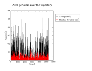
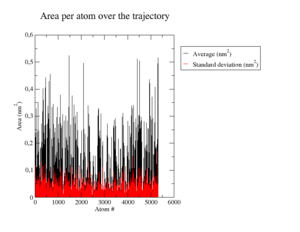
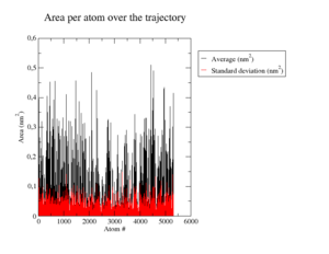
<figtable id="tab:atomic_sas">

Plot of the area of every atom accessible to the solvent during the 10 ns simulations.

a) Plot of the are aof every atom accessible to solvent of the wildtype phenylalanine hydroxylase structure 1J8U.

b) Plot of the area of every atom accessible to solvent of the Ala322Gly mutation.

c) Plot of the area of every atom accessible to solvent of the Arg408Trp mutation.

</figtable>

<figtable id="tab:residue_sas">

Plot of the area of every residue accessible to the solvent during the 10 ns simulations.

a) Plot of the are aof every residue accessible to solvent of the wildtype phenylalanine hydroxylase structure 1J8U.

b) Plot of the area of every residue accessible to solvent of the Ala322Gly mutation.

c) Plot of the area of every residue accessible to solvent of the Arg408Trp mutation.

</figtable>

• Which residues are the most accessible to the solvent?

Hydrogen Bonds

<figtable id="tab:hydrogen_bonds_protein">

Plot of the number of hydrogen bonds within the protein during the 10 ns simulations.

a) Plot of the number of hydrogen bonds within the protein of the wildtype phenylalanine hydroxylase structure 1J8U.

b) Plot of the number of hydrogen bonds within the protein of the Ala322Gly mutation.

c) Plot of the number of hydrogen bonds within the protein of the Arg408Trp mutation.

</figtable>

<figtable id="tab:hydrogen_bonds_water">

Plot of the number of hydrogen bonds from protein to water during the 10 ns simulations.

a) Plot of the number of hydrogen bonds from protein to water of the wildtype phenylalanine hydroxylase structure 1J8U.

b) Plot of the number of hydrogen bonds from protein to water of the Ala322Gly mutation.

c) Plot of the number of hydrogen bonds from protein to water of the Arg408Trp mutation.

</figtable>

• Discuss the relation between the number of hydrogen bonds for both cases and the fluctuations in each plot.

Secondary Structure

<figtable id="tab:sec_struc">

Plot of the number of residues forming secondary structure elements during the 10 ns simulations.

a) Plot of the number of residues forming secondary structure elements of the wildtype phenylalanine hydroxylase structure 1J8U.

b) Plot of the number of residues forming secondary structure elements of the Ala322Gly mutation.

c) Plot of the number of residues forming secondary structure elements of the Arg408Trp mutation.

</figtable>

<figtable id="tab:sec_struc">

Plot of the secondary structure per residue during the 10 ns simulations.

a) Plot of the the secondary structure per residue of the wildtype phenylalanine hydroxylase structure 1J8U.

b) Plot of the secondary structure per residue of the Ala322Gly mutation.

c) Plot of the secondary structure per residue of the Arg408Trp mutation.

</figtable>

• Discuss some of the changes in the secondary structure, if any.

Ramachandran Plots

• What can you say about the conformation of the residues, based on the ramachandran plots?

Analysis of Dynamics and Time-averaged Properties

Root Mean Square Deviations

<figtable id="tab:rmsd_backbone_b">

Plot of the RMSD of the backbone and the C beta atom during the 10 ns simulations.

a) Plot of the RMSD of the backbone and the C beta atom of the wildtype phenylalanine hydroxylase structure 1J8U.

b) Plot of the RMSD of the backbone and the C beta atom of the Ala322Gly mutation.

c) Plot of the RMSD of the backbone and the C beta atom of the Arg408Trp mutation.

</figtable>

<figtable id="tab:rmsd_backbone_b_matrix">

Matrix of the RMSD of the backbone and the C beta atom during the 10 ns simulations.

a) Matrix of the RMSD of the backbone and the C beta atom of the wildtype phenylalanine hydroxylase structure 1J8U.

b) Matrix of the RMSD of the backbone and the C beta atom of the Ala322Gly mutation.

c) Matrix of the RMSD of the backbone and the C beta atom of the Arg408Trp mutation.

</figtable>

• What is interesting by choosing the group "Mainchain+Cb" for this analysis?

=> Conformation and direction of residue side chain

• How many transitions do you see?
• What can you conclude from this analysis? Could you expect such a result, justify?

Cluster Analysis

• How many clusters were found and what were the sizes of the largest two?
• Are there notable differences between the two structures?

Distance RMSD

<figtable id="tab:distanec_rmsd">

Plot of the distance-RMSD of protein during the 10 ns simulations.

a) Matrix of the distance-RMSD of the wildtype phenylalanine hydroxylase structure 1J8U.

b) Matrix of the distance-RMSD of the Ala322Gly mutation.

c) Matrix of the distance-RMSD of the Arg408Trp mutation.

</figtable>

• At what time and value does the dRMSD converge and how does this graph compare to the standard RMSD?